Diffusion Anisotropy#
This notebook shows how to characterise the directional dependence of the self-diffusion coefficient D and identify the preferred diffusion pathway in a periodic crystal or porous material.
Method — spherical projection of MSD:
The 1-D diffusion coefficient along unit vector \(\hat{\mathbf{n}}\) is:
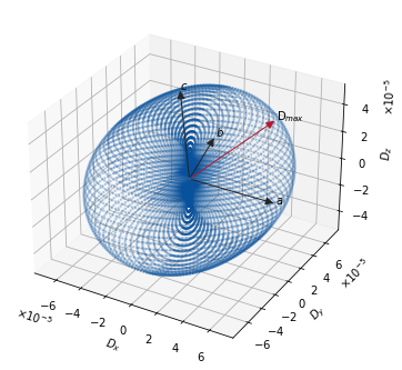
We sweep \(\hat{\mathbf{n}}\) over a spherical mesh and compute \(D_{\hat{\mathbf{n}}}\) from the slope of the projected MSD. Plotting \(D_{\hat{\mathbf{n}}} \cdot \hat{\mathbf{n}}\) as a 3-D scatter yields an anisotropy surface: its elongated axis points along the fastest diffusion channel.
Voronoi channel analysis:
Once the preferred diffusion direction is known (here ≈ [100]), the plane perpendicular to it is tessellated by Voronoi cells centred on lattice-plane reference points. Assigning each water CoM position to a Voronoi cell at every frame reveals which pore channel each molecule occupies and how often it switches channels.
Topics covered:
Loading pre-computed water CoM data
Projecting MSD along all directions on a spherical mesh
Visualising the diffusion anisotropy surface in 3-D
Voronoi tessellation to assign molecules to diffusion channels
Computing the channel-switching frequency
Import packages#
import pandas as pd
import numpy as np
import matplotlib.pyplot as plt
from cage_data import cage1_info
from fishmol.utils import vector, Arrow3D, h_channel, calc_freq
from fishmol import msd
from fishmol import style
Load water CoM data#
water_com = pd.read_excel("test/cage1-500K-water-com.xlsx", header=0, index_col=0, engine = "openpyxl")
water_com.head()
| water1_x | water1_y | water1_z | water2_x | water2_y | water2_z | water3_x | water3_y | water3_z | water4_x | ... | water5_z | water6_x | water6_y | water6_z | water7_x | water7_y | water7_z | water8_x | water8_y | water8_z | |
|---|---|---|---|---|---|---|---|---|---|---|---|---|---|---|---|---|---|---|---|---|---|
| 0 | 10.586316 | 19.902134 | 10.380009 | 0.624155 | 10.923925 | 8.298079 | -1.967392 | 4.261146 | 12.241481 | 4.693672 | ... | 4.725172 | 15.090375 | 8.649502 | 6.883228 | 17.759366 | 15.321196 | 2.865725 | 11.019290 | 3.578953 | 0.703805 |
| 1 | 10.597616 | 19.945151 | 10.393126 | 0.617881 | 10.942585 | 8.312331 | -1.961926 | 4.253910 | 12.205821 | 4.689873 | ... | 4.745156 | 15.076014 | 8.640429 | 6.849210 | 17.749958 | 15.278667 | 2.889409 | 11.049146 | 3.587807 | 0.663123 |
| 2 | 10.610208 | 20.003821 | 10.408405 | 0.610859 | 10.967922 | 8.330438 | -1.953047 | 4.243309 | 12.156421 | 4.687198 | ... | 4.767198 | 15.058083 | 8.628816 | 6.804086 | 17.738720 | 15.225162 | 2.920655 | 11.086905 | 3.600664 | 0.608757 |
| 3 | 10.622718 | 20.062112 | 10.416761 | 0.604688 | 10.993416 | 8.349495 | -1.945208 | 4.229969 | 12.106099 | 4.687512 | ... | 4.786539 | 15.040753 | 8.617851 | 6.760128 | 17.728982 | 15.181476 | 2.948253 | 11.122864 | 3.614650 | 0.558271 |
| 4 | 10.636664 | 20.122749 | 10.416813 | 0.597829 | 11.020753 | 8.373153 | -1.941190 | 4.211549 | 12.054352 | 4.691621 | ... | 4.808036 | 15.020218 | 8.605213 | 6.714651 | 17.717884 | 15.151479 | 2.970079 | 11.155729 | 3.629731 | 0.511643 |
5 rows × 24 columns
Spherical MSD Projection#
msd.proj_d() projects each water CoM trajectory onto every direction on a spherical mesh (n_phi × n_theta points), computes the 1-D MSD for each direction using the FFT algorithm, and fits a linear model to extract D. The first 1 000 frames (5 ps equilibration) are skipped before fitting.
Parameters:
df— DataFrame of CoM coordinates (columns:water{i}_x/y/z)num— number of water moleculesn_phi,n_theta— resolution of the spherical mesh (default 120 × 120)timestep— frame interval in fs (default 5 fs)
Returns vecs (unit vectors on the mesh) and ave_D (average D in cm²/s along each vector).
water_num = 8
vecs, ave_d = msd.proj_d(df = water_com, num = water_num)
Progress: [■■■■■■■■■■■■■■■■■■■■] 100.0%
data = np.concatenate((vecs, ave_d.reshape((len(vecs), 1))), axis = 1)
results = pd.DataFrame(columns = ["x", "y", "z", "mean_D"], data = data)
results.head()
| x | y | z | mean_D | |
|---|---|---|---|---|
| 0 | 1.224647e-16 | -7.498799e-33 | -1.000000 | 0.000017 |
| 1 | 5.277535e-02 | -3.231558e-18 | -0.998606 | 0.000018 |
| 2 | 1.054036e-01 | -6.454109e-18 | -0.994430 | 0.000019 |
| 3 | 1.577381e-01 | -9.658671e-18 | -0.987481 | 0.000020 |
| 4 | 2.096329e-01 | -1.283631e-17 | -0.977780 | 0.000022 |
results.to_excel("test/cage1-500K-aniso.xlsx")
cell= [
    [21.2944000000,        0.0000000000,        0.0000000000],
    [-4.6030371123,       20.7909480472,        0.0000000000],
    [-0.9719093466,       -1.2106211379,       15.1054299403]
]

diags = [[1,0,0],[0,1,0],[0,0,1]]
diags = [ vector(diag, cell = cell, name = "m") for diag in diags]
[diag.to_cart() for diag in diags]
[<fishmol.utils.vector at 0x7fd125c34c10>,
 <fishmol.utils.vector at 0x7fd125c34bb0>,
 <fishmol.utils.vector at 0x7fd125c34d00>]
x = vecs[:,0]*ave_d
y = vecs[:,1]*ave_d
z = vecs[:,2]*ave_d
# ave_d = data.iloc[:,3].to_numpy()
fig = plt.figure(figsize = (5, 4.6))
ax = fig.add_axes([0.0,0.04,0.90,0.96], projection='3d')

zdirs = (None,)*3
labels = ("$a$", "$b$", "$c$")

# ax.plot_trisurf(x, y, z, edgecolor ='none', cmap='PuBu', alpha=0.8)
ax.scatter3D(x, y, z, edgecolor ='none', marker = ".", color = "#08519c", alpha=0.3)

for i, axis in enumerate(diags):
    axis = axis.array/15000
    a = Arrow3D([0, axis[0]], [0, axis[1]], [0, axis[2]], mutation_scale=15,
            lw=1, arrowstyle="-|>", color="#252525")
    ax.add_artist(a)
    ax.text(*axis, labels[i], zdirs[i])

idx = np.where(ave_d == np.amax(ave_d))
h_path = vecs[idx]*ave_d[idx]

a = Arrow3D(*zip(np.zeros(3), h_path[0]), mutation_scale=15,
        lw=1, arrowstyle="-|>", color="#b2182b")
ax.add_artist(a)
ax.text(*h_path[0], "D$_{max}$", None)

ax.set_xlabel("$D_x$")
ax.set_ylabel("$D_y$")
ax.set_zlabel("$D_z$")

ax.ticklabel_format(axis='both', style='sci', scilimits=[-4,4], useMathText=True)

plt.savefig("test/cage1-aniso-500K.jpg", dpi = 600)

plt.show()
/tmp/ipykernel_3339671/2059225541.py:31: MatplotlibDeprecationWarning: The 'renderer' parameter of do_3d_projection() was deprecated in Matplotlib 3.4 and will be removed two minor releases later.
  plt.savefig("test/cage1-aniso-500K.jpg", dpi = 600)
Voronoi Channel Analysis#
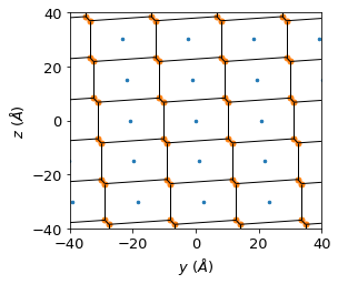
Once the dominant diffusion direction is identified (here [100], i.e. along a), we project the problem onto the perpendicular b–c plane and use a Voronoi tessellation to partition that plane into diffusion channels.
Reference points for the Voronoi cells are chosen as a regular grid of integer Miller index positions in the b–c plane (e.g. (0, m, n) for various m, n). Each reference point corresponds to one pore channel. At each frame, the CoM position of a water molecule is assigned to its nearest Voronoi cell, giving a time series of channel labels.
calc_freq(out, timestep=5) counts the number of times the channel label changes and divides by the total simulation time to give the switching frequency in ps⁻¹.
Cage 1 500 K#
The h-path is almost aligned with [100], and the following points used to devide channels
points = np.asarray([
    (0, -3, -2), (0, -3, -1), (0, -3, 0), (0, -3, 1), (0, -3, 2), (0, -3, 3),
    (0, -2, -3), (0, -2, -2), (0, -2, -1), (0, -2, 0), (0, -2, 1), (0, -2, 2), (0, -2, 3),
    (0, -1, -3), (0, -1, -2), (0, -1, -1), (0, -1, 0), (0, -1, 1), (0, -1, 2), (0, -1, 3),
    (0, 0, -3), (0, 0, -2), (0, 0, -1), (0, 0, 0), (0, 0, 1), (0, 0, 2), (0, 0, 3),
    (0, 1, -3), (0, 1, -2), (0, 1, -1), (0, 1, 0), (0, 1, 1), (0, 1, 2), (0, 1, 3),
    (0, 2, -3), (0, 2, -2), (0, 2, -1), (0, 2, 0), (0, 2, 1), (0, 2, 2), (0, 2, 3),
    (0, 3, -2), (0, 3, -1), (0, 3, 0), (0, 3, 1), (0, 3, 2), (0, 3, 3)
], dtype = np.float64)

cell = cage1_info.cell

# The coordination the points will be projected to new coordinate system, where w3 is the h_path with the highest proton diffusivity
w1 = vector([0, 1, 0], cell = cell, name = "m")
w2 = vector([0, 0, 1], cell = cell, name = "m")
w3 = vector([1, 0, 0], cell = cell, name = "m")

W = np.asarray([globals()[f'w{i + 1}'].array for i in range(3)])
points_arrs = [vector(point, cell = cell) for point in points]
for point_arr in points_arrs:
    point_arr.to_cart(normalise = False)
points = np.asarray([point.array for point in points_arrs])
points
array([[ 15.75293003, -59.95160187, -30.21085988],
       [ 14.78102068, -61.162223  , -15.10542994],
       [ 13.80911134, -62.37284414,   0.        ],
       [ 12.83720199, -63.58346528,  15.10542994],
       [ 11.86529264, -64.79408642,  30.21085988],
       [ 10.8933833 , -66.00470756,  45.31628982],
       [ 12.12180226, -37.95003268, -45.31628982],
       [ 11.14989292, -39.16065382, -30.21085988],
       [ 10.17798357, -40.37127496, -15.10542994],
       [  9.20607422, -41.58189609,   0.        ],
       [  8.23416488, -42.79251723,  15.10542994],
       [  7.26225553, -44.00313837,  30.21085988],
       [  6.29034618, -45.21375951,  45.31628982],
       [  7.51876515, -17.15908463, -45.31628982],
       [  6.54685581, -18.36970577, -30.21085988],
       [  5.57494646, -19.58032691, -15.10542994],
       [  4.60303711, -20.79094805,   0.        ],
       [  3.63112777, -22.00156919,  15.10542994],
       [  2.65921842, -23.21219032,  30.21085988],
       [  1.68730907, -24.42281146,  45.31628982],
       [  2.91572804,   3.63186341, -45.31628982],
       [  1.94381869,   2.42124228, -30.21085988],
       [  0.97190935,   1.21062114, -15.10542994],
       [  0.        ,   0.        ,   0.        ],
       [ -0.97190935,  -1.21062114,  15.10542994],
       [ -1.94381869,  -2.42124228,  30.21085988],
       [ -2.91572804,  -3.63186341,  45.31628982],
       [ -1.68730907,  24.42281146, -45.31628982],
       [ -2.65921842,  23.21219032, -30.21085988],
       [ -3.63112777,  22.00156919, -15.10542994],
       [ -4.60303711,  20.79094805,   0.        ],
       [ -5.57494646,  19.58032691,  15.10542994],
       [ -6.54685581,  18.36970577,  30.21085988],
       [ -7.51876515,  17.15908463,  45.31628982],
       [ -6.29034618,  45.21375951, -45.31628982],
       [ -7.26225553,  44.00313837, -30.21085988],
       [ -8.23416488,  42.79251723, -15.10542994],
       [ -9.20607422,  41.58189609,   0.        ],
       [-10.17798357,  40.37127496,  15.10542994],
       [-11.14989292,  39.16065382,  30.21085988],
       [-12.12180226,  37.95003268,  45.31628982],
       [-11.86529264,  64.79408642, -30.21085988],
       [-12.83720199,  63.58346528, -15.10542994],
       [-13.80911134,  62.37284414,   0.        ],
       [-14.78102068,  61.162223  ,  15.10542994],
       [-15.75293003,  59.95160187,  30.21085988],
       [-16.72483938,  58.74098073,  45.31628982]])
from scipy.spatial import voronoi_plot_2d
vor = h_channel(points[:,1:])
fig = voronoi_plot_2d(vor)
ax = plt.gca()

ax.set_xlim(-40,40)
ax.set_ylim(-40,40)

ax.set_xlabel("$y$ ($\AA$)")
ax.set_ylabel("$z$ ($\AA$)")
plt.show()
Load CoM data
# y-z CoM coordinates of water 1 (the one whose channel we track)
water1 = water_com.iloc[:, 1:3].to_numpy()

# Assign each frame's position to the nearest Voronoi region
out = np.asarray(vor.sort_points(water1))

# Group frame positions by region index using a dict (avoids namespace pollution)
regions = {}
for n in vor.point_region:
    idx = np.where(out == n)
    regions[n] = water1[idx]
Calculate the frequency of switch channels#
The water molecule stayed inside the diffusion channel as we used a small part of our simulation data
# calc_freq returns channel-switching events per ps
# timestep=5 fs must be passed explicitly to match the trajectory output frequency
freq = calc_freq(out, timestep=5)
print(f"Channel-switching frequency: {freq:.4f} ps⁻¹")
fig = voronoi_plot_2d(vor)
ax = plt.gca()

for n, pts in regions.items():
    if pts.size > 0:
        ax.scatter(pts[:, 0], pts[:, 1], s=30, linewidths=0, alpha=0.1, zorder=0)

ax.set_xlim(-40, 40)
ax.set_ylim(-40, 40)
ax.set_xlabel("$y$ ($\\AA$)")
ax.set_ylabel("$z$ ($\\AA$)")
plt.show()