SHAP

Contents cliped from the book Interpretable Machine Learning - A Guide for Making Black Box Models Explainable View the original book chapter here: christophm.github.io

Shapley Values

A prediction can be explained by assuming that each feature value of the instance is a “player” in a game where the prediction is the payout. Shapley values – a method from coalitional game theory – tells us how to fairly distribute the “payout” among the features.

General Idea

Assume the following scenario:

You have trained a machine learning model to predict apartment prices. For a certain apartment it predicts €300,000 and you need to explain this prediction. The apartment has an area of 50 m$^2$, is located on the 2nd floor, has a park nearby and cats are banned:

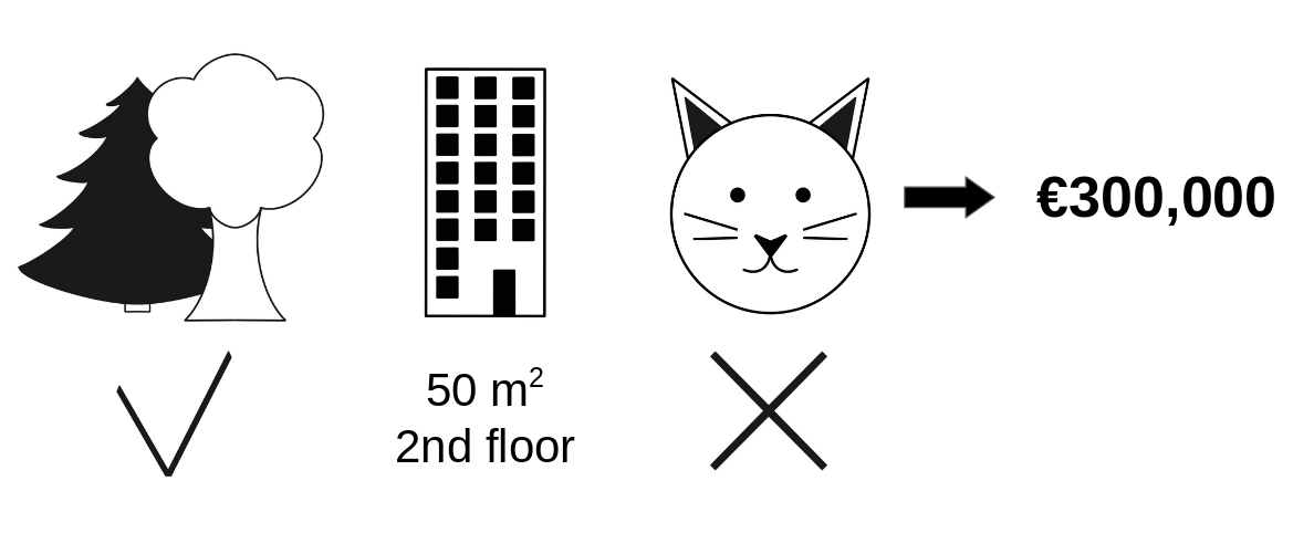
FIGURE 9.17: The predicted price for a 50 m$^2$ 2nd floor apartment with a nearby park and cat ban is €300,000. Our goal is to explain how each of these feature values contributed to the prediction.

The average prediction for all apartments is €310,000. How much has each feature value contributed to the prediction compared to the average prediction?

The answer is simple for linear regression models: the effect of each feature is the weight of the feature times the feature value, because of the linearity. For more complex models, we need a different solution. For example, LIME suggests local models to estimate effects. Another solution comes from cooperative game theory: The Shapley value, coined by Shapley (1953)63, is a method for assigning payouts to players depending on their contribution to the total payout. Players cooperate in a coalition and receive a certain profit from this cooperation.

Players? Game? Payout? What is the connection to machine learning predictions and interpretability? The “game” is the prediction task for a single instance of the dataset. The “gain” is the actual prediction for this instance minus the average prediction for all instances. The “players” are the feature values of the instance that collaborate to receive the gain (= predict a certain value). In our apartment example, the feature values park-nearby, cat-banned, area-50 and floor-2nd worked together to achieve the prediction of €300,000. Our goal is to explain the difference between the actual prediction (€300,000) and the average prediction (€310,000): a difference of -€10,000.

The answer could be: The park-nearby contributed €30,000; area-50 contributed €10,000; floor-2nd contributed €0; cat-banned contributed -€50,000. The contributions add up to -€10,000, the final prediction minus the average predicted apartment price.

How do we calculate the Shapley value for one feature?

The Shapley value is the average marginal contribution of a feature value across all possible coalitions. All clear now?

In the following figure we evaluate the contribution of the cat-banned feature value when it is added to a coalition of park-nearby and area-50. We simulate that only park-nearby, cat-banned and area-50 are in a coalition by randomly drawing another apartment from the data and using its value for the floor feature. The value floor-2nd was replaced by the randomly drawn floor-1st. Then we predict the price of the apartment with this combination (€310,000). In a second step, we remove cat-banned from the coalition by replacing it with a random value of the cat allowed/banned feature from the randomly drawn apartment. In the example it was cat-allowed, but it could have been cat-banned again. We predict the apartment price for the coalition of park-nearby and area-50 (€320,000). The contribution of cat-banned was €310,000 - €320,000 = -€10,000. This estimate depends on the values of the randomly drawn apartment that served as a “donor” for the cat and floor feature values. We will get better estimates if we repeat this sampling step and average the contributions.

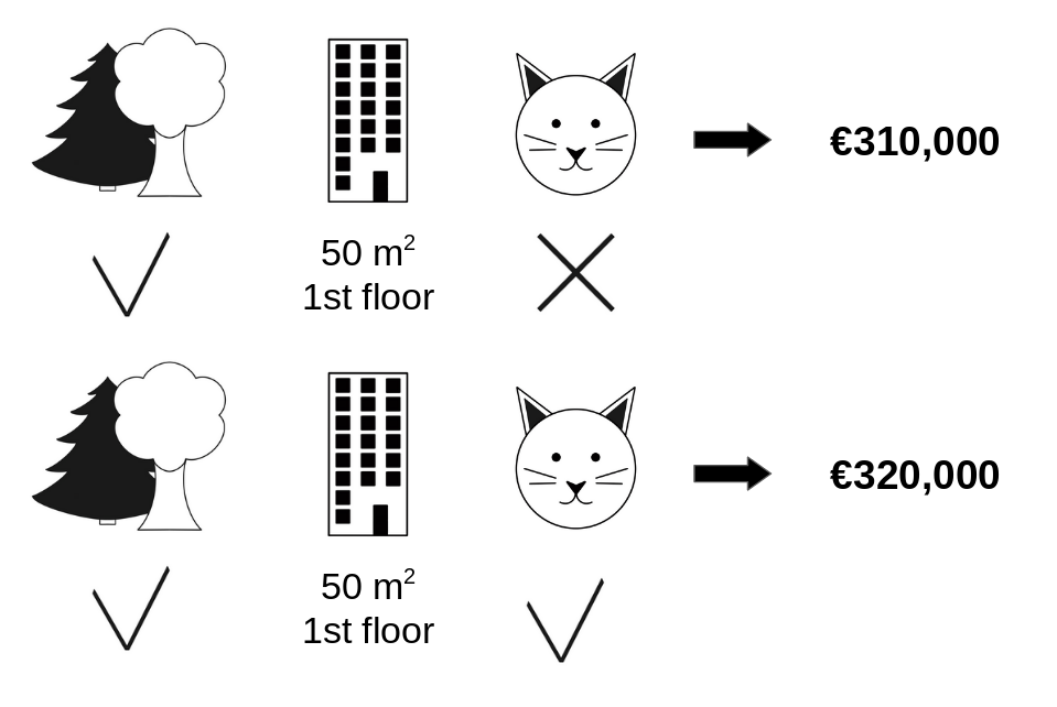
FIGURE 9.18: One sample repetition to estimate the contribution of cat-banned to the prediction when added to the coalition of park-nearby and area-50.

We repeat this computation for all possible coalitions. The Shapley value is the average of all the marginal contributions to all possible coalitions. The computation time increases exponentially with the number of features. One solution to keep the computation time manageable is to compute contributions for only a few samples of the possible coalitions.

The following figure shows all coalitions of feature values that are needed to determine the Shapley value for cat-banned. The first row shows the coalition without any feature values. The second, third and fourth rows show different coalitions with increasing coalition size, separated by “|”. All in all, the following coalitions are possible:

• No feature values
• park-nearby
• area-50
• floor-2nd
• park-nearby+area-50
• park-nearby+floor-2nd
• area-50+floor-2nd
• park-nearby+area-50+floor-2nd.

For each of these coalitions we compute the predicted apartment price with and without the feature value cat-banned and take the difference to get the marginal contribution. The Shapley value is the (weighted) average of marginal contributions. We replace the feature values of features that are not in a coalition with random feature values from the apartment dataset to get a prediction from the machine learning model.

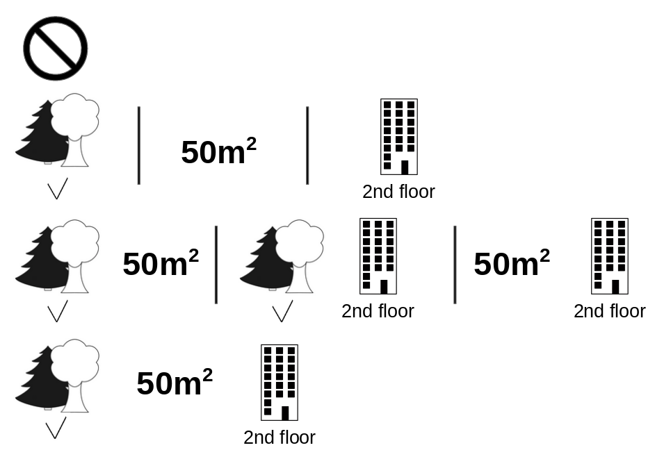
FIGURE 9.19: All 8 coalitions needed for computing the exact Shapley value of the cat-banned feature value.

If we estimate the Shapley values for all feature values, we get the complete distribution of the prediction (minus the average) among the feature values.

Examples and Interpretation

The interpretation of the Shapley value for feature value $j$ is: The value of the $j$-th feature contributed $\phi_j$ to the prediction of this particular instance compared to the average prediction for the dataset.

The Shapley value works for both classification (if we are dealing with probabilities) and regression.

We use the Shapley value to analyze the predictions of a random forest model predicting cervical cancer:

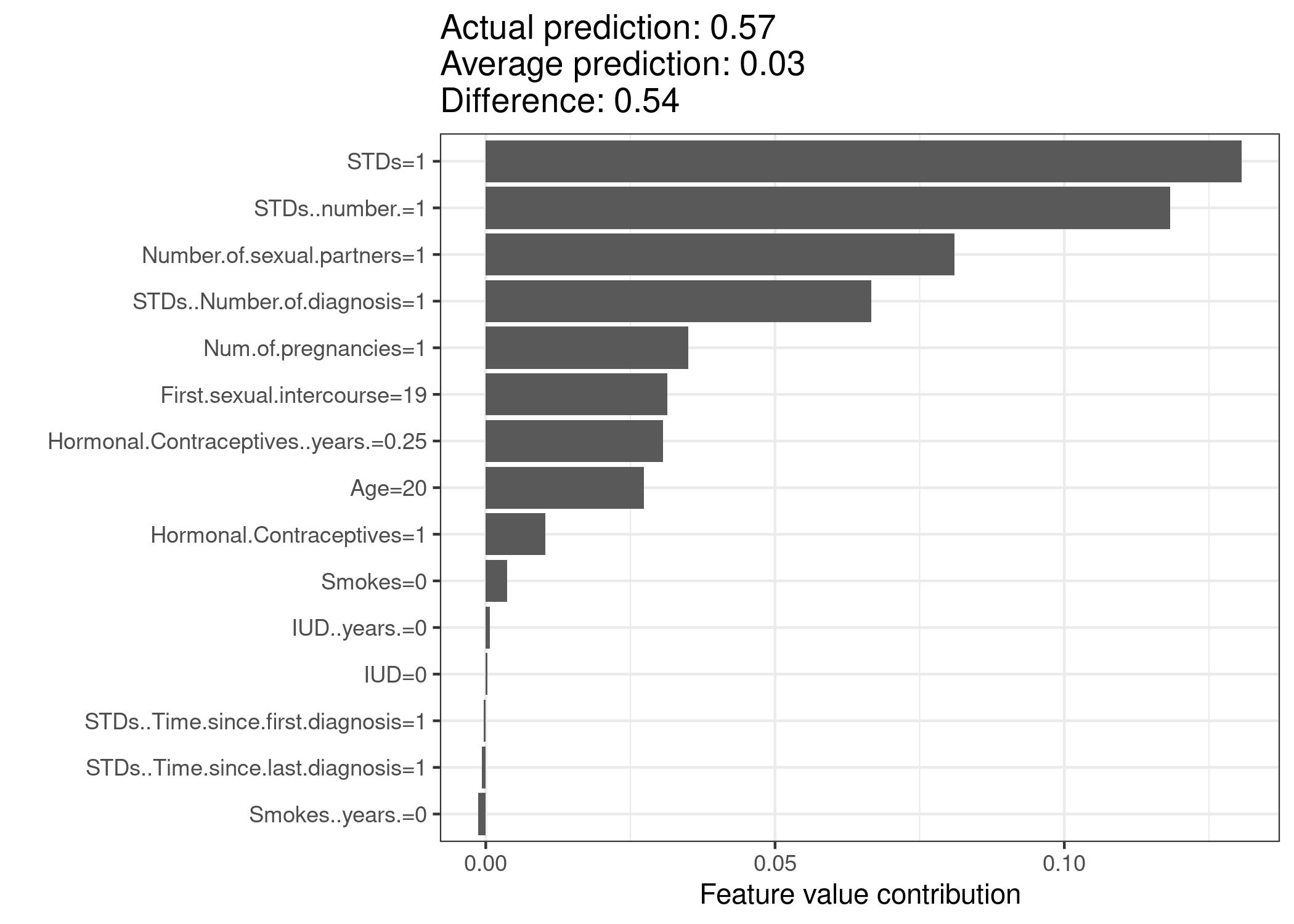
FIGURE 9.20: Shapley values for a woman in the cervical cancer dataset. With a prediction of 0.57, this woman’s cancer probability is 0.54 above the average prediction of 0.03. The number of diagnosed STDs increased the probability the most. The sum of contributions yields the difference between actual and average prediction (0.54).

For the bike rental dataset, we also train a random forest to predict the number of rented bikes for a day, given weather and calendar information. The explanations created for the random forest prediction of a particular day:

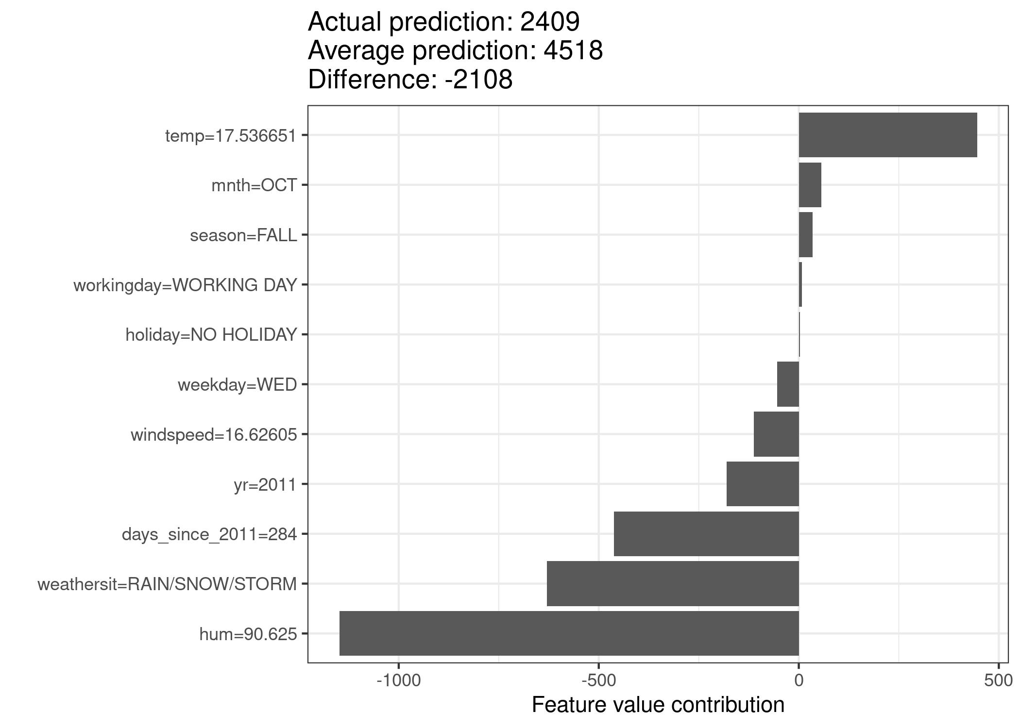
FIGURE 9.21: Shapley values for day 285. With a predicted 2409 rental bikes, this day is -2108 below the average prediction of 4518. The weather situation and humidity had the largest negative contributions. The temperature on this day had a positive contribution. The sum of Shapley values yields the difference of actual and average prediction (-2108).

Be careful to interpret the Shapley value correctly: The Shapley value is the average contribution of a feature value to the prediction in different coalitions. The Shapley value is NOT the difference in prediction when we would remove the feature from the model.

The Shapley Value in Detail

This section goes deeper into the definition and computation of the Shapley value for the curious reader. Skip this section and go directly to “Advantages and Disadvantages” if you are not interested in the technical details.

We are interested in how each feature affects the prediction of a data point. In a linear model it is easy to calculate the individual effects. Here is what a linear model prediction looks like for one data instance:

where $x$ is the instance for which we want to compute the contributions. Each $x_j$ is a feature value, with j = 1,…,p. The $\beta_j$ is the weight corresponding to feature j.

The contribution $\phi_j$ of the j-th feature on the prediction $\hat{f}(x)$ is:

where $E(\beta_jX_{j})$ is the mean effect estimate for feature j. The contribution is the difference between the feature effect minus the average effect. Nice! Now we know how much each feature contributed to the prediction. If we sum all the feature contributions for one instance, the result is the following:

This is the predicted value for the data point x minus the average predicted value. Feature contributions can be negative.

Can we do the same for any type of model? It would be great to have this as a model-agnostic tool. Since we usually do not have similar weights in other model types, we need a different solution.

Help comes from unexpected places: cooperative game theory. The Shapley value is a solution for computing feature contributions for single predictions for any machine learning model.

The Shapley Value

The Shapley value is defined via a value function $val$ of players in S.

The Shapley value of a feature value is its contribution to the payout, weighted and summed over all possible feature value combinations:

where S is a subset of the features used in the model, x is the vector of feature values of the instance to be explained and p the number of features. $val_x(S)$ is the prediction for feature values in set S that are marginalized over features that are not included in set S:

You actually perform multiple integrations for each feature that is not contained S. A concrete example: The machine learning model works with 4 features x1, x2, x3 and x4 and we evaluate the prediction for the coalition S consisting of feature values x1 and x3:

This looks similar to the feature contributions in the linear model!

Do not get confused by the many uses of the word “value”: The feature value is the numerical or categorical value of a feature and instance; the Shapley value is the feature contribution to the prediction; the value function is the payout function for coalitions of players (feature values).

The Shapley value is the only attribution method that satisfies the properties Efficiency, Symmetry, Dummy and Additivity, which together can be considered a definition of a fair payout.

Efficiency The feature contributions must add up to the difference of prediction for x and the average.

Symmetry The contributions of two feature values j and k should be the same if they contribute equally to all possible coalitions. If

for all

then

Dummy A feature j that does not change the predicted value – regardless of which coalition of feature values it is added to – should have a Shapley value of 0. If

for all

then

Additivity For a game with combined payouts val+val+ the respective Shapley values are as follows:

Suppose you trained a random forest, which means that the prediction is an average of many decision trees. The Additivity property guarantees that for a feature value, you can calculate the Shapley value for each tree individually, average them, and get the Shapley value for the feature value for the random forest.

Intuition

An intuitive way to understand the Shapley value is the following illustration: The feature values enter a room in random order. All feature values in the room participate in the game (= contribute to the prediction). The Shapley value of a feature value is the average change in the prediction that the coalition already in the room receives when the feature value joins them.

Estimating the Shapley Value

All possible coalitions (sets) of feature values have to be evaluated with and without the j-th feature to calculate the exact Shapley value. For more than a few features, the exact solution to this problem becomes problematic as the number of possible coalitions exponentially increases as more features are added. Strumbelj et al. (2014)64 propose an approximation with Monte-Carlo sampling:

where $\hat{f} (x^m_{+j})$ is the prediction for $x$, but with a random number of feature values replaced by feature values from a random data point $z$, except for the respective value of feature $j$. The $x$-vector $x^m_{-j}$ is almost identical to $x^m_{+j}$, but the value $x^m_j$ is also taken from the sampled $z$. Each of these M new instances is a kind of “Frankenstein’s Monster” assembled from two instances. Note that in the following algorithm, the order of features is not actually changed – each feature remains at the same vector position when passed to the predict function. The order is only used as a “trick” here: By giving the features a new order, we get a random mechanism that helps us put together the “Frankenstein’s Monster”. For features that appear left of the feature $x_j$, we take the values from the original observations, and for the features on the right, we take the values from a random instance.

Approximate Shapley estimation for single feature value:

• Output: Shapley value for the value of the j-th feature
• Required: Number of iterations M, instance of interest x, feature index j, data matrix X, and machine learning model f
  • For all m = 1,…,M:
    • Draw random instance z from the data matrix X
    • Choose a random permutation o of the feature values
    • Order instance x: $x_o=(x_{(1)},\ldots,x_{(j)},\ldots,x_{(p)})$
    • Order instance z: $z_o=(z_{(1)},\ldots,z_{(j)},\ldots,z_{(p)})$
    • Construct two new instances
      • With j: $x_{+j}=(x_{(1)},\ldots,x_{(j-1)},x_{(j)},z_{(j+1)},\ldots,z_{(p)})$
      • Without j: $x_{-j}=(x_{(1)},\ldots,x_{(j-1)},z_{(j)},z_{(j+1)},\ldots,z_{(p)})$
    • Compute marginal contribution: $\phi_j^{m}=\hat{f}(x_{+j})-\hat{f}(x_{-j})$
• Compute Shapley value as the average: $\phi_j(x)=\frac{1}{M}\sum_{m=1}^M\phi_j^{m}$

First, select an instance of interest x, a feature j and the number of iterations M. For each iteration, a random instance z is selected from the data and a random order of the features is generated. Two new instances are created by combining values from the instance of interest x and the sample z. The instance $x_{+j}$ is the instance of interest, but all values in the order after feature j are replaced by feature values from the sample z. The instance $x_{-j}$ is the same as $x_{+j}$, but in addition has feature j replaced by the value for feature j from the sample z. The difference in the prediction from the black box is computed:

All these differences are averaged and result in:

Averaging implicitly weighs samples by the probability distribution of X.

The procedure has to be repeated for each of the features to get all Shapley values.

Advantages

The difference between the prediction and the average prediction is fairly distributed among the feature values of the instance – the Efficiency property of Shapley values. This property distinguishes the Shapley value from other methods such as LIME. LIME does not guarantee that the prediction is fairly distributed among the features. The Shapley value might be the only method to deliver a full explanation. In situations where the law requires explainability – like EU’s “right to explanations” – the Shapley value might be the only legally compliant method, because it is based on a solid theory and distributes the effects fairly. I am not a lawyer, so this reflects only my intuition about the requirements.

The Shapley value allows contrastive explanations. Instead of comparing a prediction to the average prediction of the entire dataset, you could compare it to a subset or even to a single data point. This contrastiveness is also something that local models like LIME do not have.

The Shapley value is the only explanation method with a solid theory. The axioms – efficiency, symmetry, dummy, additivity – give the explanation a reasonable foundation. Methods like LIME assume linear behavior of the machine learning model locally, but there is no theory as to why this should work.

It is mind-blowing to explain a prediction as a game played by the feature values.

Disadvantages

The Shapley value requires a lot of computing time. In 99.9% of real-world problems, only the approximate solution is feasible. An exact computation of the Shapley value is computationally expensive because there are 2k possible coalitions of the feature values and the “absence” of a feature has to be simulated by drawing random instances, which increases the variance for the estimate of the Shapley values estimation. The exponential number of the coalitions is dealt with by sampling coalitions and limiting the number of iterations M. Decreasing M reduces computation time, but increases the variance of the Shapley value. There is no good rule of thumb for the number of iterations M. M should be large enough to accurately estimate the Shapley values, but small enough to complete the computation in a reasonable time. It should be possible to choose M based on Chernoff bounds, but I have not seen any paper on doing this for Shapley values for machine learning predictions.

The Shapley value can be misinterpreted. The Shapley value of a feature value is not the difference of the predicted value after removing the feature from the model training. The interpretation of the Shapley value is: Given the current set of feature values, the contribution of a feature value to the difference between the actual prediction and the mean prediction is the estimated Shapley value.

The Shapley value is the wrong explanation method if you seek sparse explanations (explanations that contain few features). Explanations created with the Shapley value method always use all the features. Humans prefer selective explanations, such as those produced by LIME. LIME might be the better choice for explanations lay-persons have to deal with. Another solution is SHAP introduced by Lundberg and Lee (2016)65, which is based on the Shapley value, but can also provide explanations with few features.

The Shapley value returns a simple value per feature, but no prediction model like LIME. This means it cannot be used to make statements about changes in prediction for changes in the input, such as: “If I were to earn €300 more a year, my credit score would increase by 5 points.”

Another disadvantage is that you need access to the data if you want to calculate the Shapley value for a new data instance. It is not sufficient to access the prediction function because you need the data to replace parts of the instance of interest with values from randomly drawn instances of the data. This can only be avoided if you can create data instances that look like real data instances but are not actual instances from the training data.

Like many other permutation-based interpretation methods, the Shapley value method suffers from inclusion of unrealistic data instances when features are correlated. To simulate that a feature value is missing from a coalition, we marginalize the feature. This is achieved by sampling values from the feature’s marginal distribution. This is fine as long as the features are independent. When features are dependent, then we might sample feature values that do not make sense for this instance. But we would use those to compute the feature’s Shapley value. One solution might be to permute correlated features together and get one mutual Shapley value for them. Another adaptation is conditional sampling: Features are sampled conditional on the features that are already in the team. While conditional sampling fixes the issue of unrealistic data points, a new issue is introduced: The resulting values are no longer the Shapley values to our game, since they violate the symmetry axiom, as found out by Sundararajan et al. (2019)66 and further discussed by Janzing et al. (2020)67.

Software and Alternatives

Shapley values are implemented in both the iml and fastshap packages for R. In Julia, you can use Shapley.jl.

SHAP, an alternative estimation method for Shapley values, is presented in the next chapter.

Another approach is called breakDown, which is implemented in the breakDown R package68. BreakDown also shows the contributions of each feature to the prediction, but computes them step by step. Let us reuse the game analogy: We start with an empty team, add the feature value that would contribute the most to the prediction and iterate until all feature values are added. How much each feature value contributes depends on the respective feature values that are already in the “team”, which is the big drawback of the breakDown method. It is faster than the Shapley value method, and for models without interactions, the results are the same.

SHAP (SHapley Additive Explanations)

Contents cliped from the book Interpretable Machine Learning - A Guide for Making Black Box Models Explainable View the original book chapter here: christophm.github.io

SHAP (SHapley Additive exPlanations) by Lundberg and Lee (2017)69 is a method to explain individual predictions. SHAP is based on the game theoretically optimal Shapley values.

There are two reasons why SHAP got its own chapter and is not a subchapter of Shapley values. First, the SHAP authors proposed KernelSHAP, an alternative, kernel-based estimation approach for Shapley values inspired by local surrogate models. And they proposed TreeSHAP, an efficient estimation approach for tree-based models. Second, SHAP comes with many global interpretation methods based on aggregations of Shapley values. This chapter explains both the new estimation approaches and the global interpretation methods.

Just looking for the correct interpretation of SHAP lots? Save yourself time and get the SHAP plots cheat sheet.

I recommend reading the chapters on Shapley values and local models (LIME) first.

Definition

The goal of SHAP is to explain the prediction of an instance x by computing the contribution of each feature to the prediction. The SHAP explanation method computes Shapley values from coalitional game theory. The feature values of a data instance act as players in a coalition. Shapley values tell us how to fairly distribute the “payout” (= the prediction) among the features. A player can be an individual feature value, e.g. for tabular data. A player can also be a group of feature values. For example to explain an image, pixels can be grouped to superpixels and the prediction distributed among them. One innovation that SHAP brings to the table is that the Shapley value explanation is represented as an additive feature attribution method, a linear model. That view connects LIME and Shapley values. SHAP specifies the explanation as:

where g is the explanation model, $z’\in{0,1}^M$ is the coalition vector, M is the maximum coalition size and $\phi_j\in\mathbb{R}$ is the feature attribution for a feature j, the Shapley values. What I call “coalition vector” is called “simplified features” in the SHAP paper. I think this name was chosen, because for e.g. image data, the images are not represented on the pixel level, but aggregated to superpixels. I believe it is helpful to think about the z’s as describing coalitions: In the coalition vector, an entry of 1 means that the corresponding feature value is “present” and 0 that it is “absent”. This should sound familiar to you if you know about Shapley values. To compute Shapley values, we simulate that only some feature values are playing (“present”) and some are not (“absent”). The representation as a linear model of coalitions is a trick for the computation of the $\phi$’s. For x, the instance of interest, the coalition vector x’ is a vector of all 1’s, i.e. all feature values are “present”. The formula simplifies to:

You can find this formula in similar notation in the Shapley value chapter. More about the actual estimation comes later. Let us first talk about the properties of the $\phi$’s before we go into the details of their estimation.

Shapley values are the only solution that satisfies properties of Efficiency, Symmetry, Dummy and Additivity. SHAP also satisfies these, since it computes Shapley values. In the SHAP paper, you will find discrepancies between SHAP properties and Shapley properties. SHAP describes the following three desirable properties:

1) Local accuracy

If you define $\phi_0=E_X(\hat{f}(x))$ and set all $x_j’$ to 1, this is the Shapley efficiency property. Only with a different name and using the coalition vector.

2) Missingness

Missingness says that a missing feature gets an attribution of zero. Note that $x_j’$ refers to the coalitions where a value of 0 represents the absence of a feature value. In coalition notation, all feature values $x_j’$ of the instance to be explained should be ‘1’. The presence of a 0 would mean that the feature value is missing for the instance of interest. This property is not among the properties of the “normal” Shapley values. So why do we need it for SHAP? Lundberg calls it a “minor book-keeping property”. A missing feature could – in theory – have an arbitrary Shapley value without hurting the local accuracy property, since it is multiplied with $x_j’=0$. The Missingness property enforces that missing features get a Shapley value of 0. In practice, this is only relevant for features that are constant.

3) Consistency

Let $\hat{f} x (z’) = \hat{f} (h_x (z’))$, and $z{-j}’$ indicate that $z_j’=0$. For any two models f and f’ that satisfy:

for all inputs $z’\in{0,1}^M$, then:

The consistency property says that if a model changes so that the marginal contribution of a feature value increases or stays the same (regardless of other features), the Shapley value also increases or stays the same. From Consistency the Shapley properties Linearity, Dummy and Symmetry follow, as described in the Appendix of Lundberg and Lee.

KernelSHAP

KernelSHAP estimates for an instance x the contributions of each feature value to the prediction. KernelSHAP consists of five steps:

• Sample coalitions $z_k’\in{0,1}^M,\quad{}k\in{1,\ldots,K}$ (1 = feature present in coalition, 0 = feature absent).
• Get prediction for each $z_k’$ by first converting $z_k’$ to the original feature space and then applying model $\hat{f}: \hat{f}(h_x(z_k’))$
• Compute the weight for each $z_k’$ with the SHAP kernel.
• Fit weighted linear model.
• Return Shapley values $\phi_k$, the coefficients from the linear model.

We can create a random coalition by repeated coin flips until we have a chain of 0’s and 1’s. For example, the vector of (1,0,1,0) means that we have a coalition of the first and third features. The K sampled coalitions become the dataset for the regression model. The target for the regression model is the prediction for a coalition. (“Hold on!,” you say. “The model has not been trained on these binary coalition data and cannot make predictions for them.”) To get from coalitions of feature values to valid data instances, we need a function $h_x(z’)=z$ where $h_x:{0,1}^M\rightarrow\mathbb{R}^p$. The function $h_x$ maps 1’s to the corresponding value from the instance x that we want to explain. For tabular data, it maps 0’s to the values of another instance that we sample from the data. This means that we equate “feature value is absent” with “feature value is replaced by random feature value from data”. For tabular data, the following figure visualizes the mapping from coalitions to feature values:

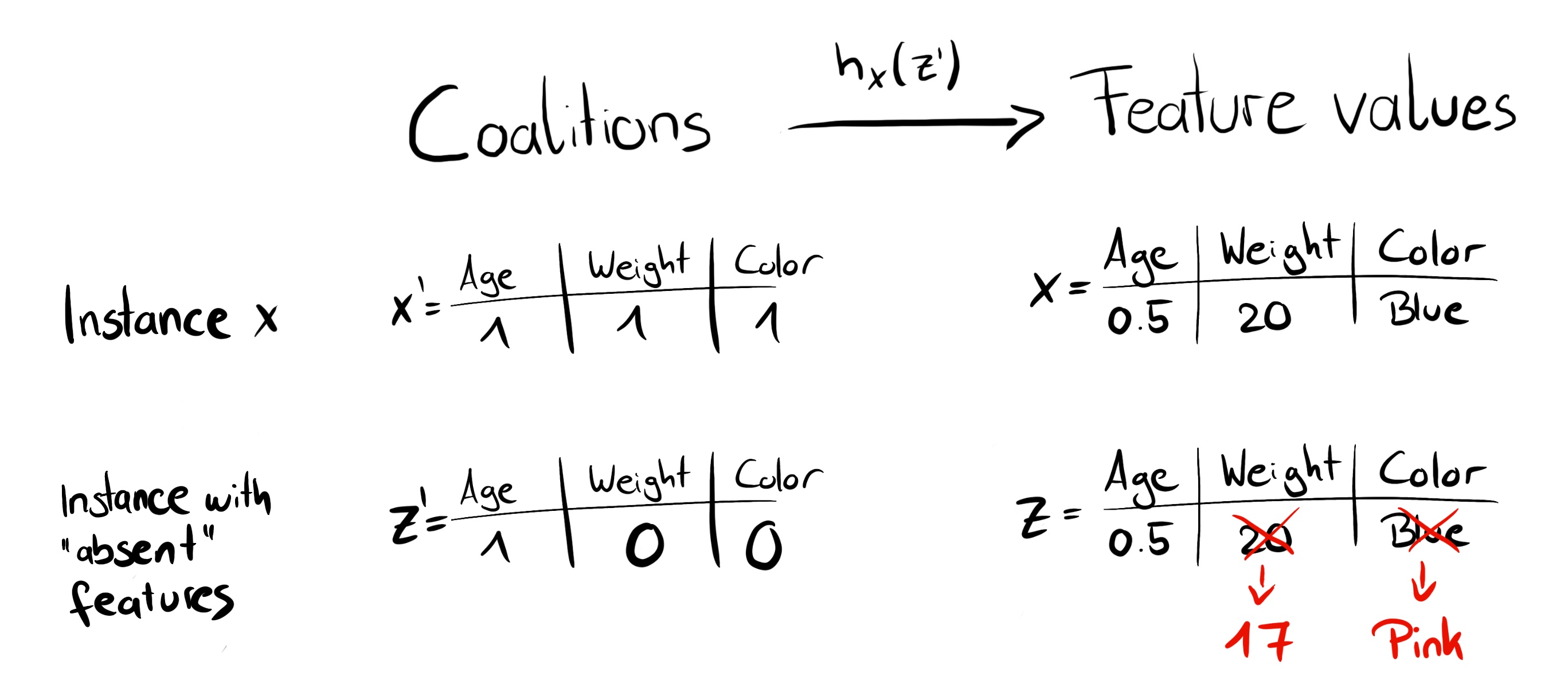
FIGURE 9.22: Function $h_x$ maps a coalition to a valid instance. For present features (1), $h_x$ maps to the feature values of x. For absent features (0), $h_x$ maps to the values of a randomly sampled data instance.

$h_x$ for tabular data treats feature $X_j$ and $X_{-j}$ (the other features) as independent and integrates over the marginal distribution:

Sampling from the marginal distribution means ignoring the dependence structure between present and absent features. KernelSHAP therefore suffers from the same problem as all permutation-based interpretation methods. The estimation puts too much weight on unlikely instances. Results can become unreliable. But it is necessary to sample from the marginal distribution. The solution would be to sample from the conditional distribution, which changes the value function, and therefore the game to which Shapley values are the solution. As a result, the Shapley values have a different interpretation: For example, a feature that might not have been used by the model at all can have a non-zero Shapley value when the conditional sampling is used. For the marginal game, this feature value would always get a Shapley value of 0, because otherwise it would violate the Dummy axiom.

For images, the following figure describes a possible mapping function:

FIGURE 9.23: Function $h_x$ maps coalitions of superpixels (sp) to images. Superpixels are groups of pixels. For present features (1), $h_x$ returns the corresponding part of the original image. For absent features (0), $h_x$ greys out the corresponding area. Assigning the average color of surrounding pixels or similar would also be an option.

The big difference to LIME is the weighting of the instances in the regression model. LIME weights the instances according to how close they are to the original instance. The more 0’s in the coalition vector, the smaller the weight in LIME. SHAP weights the sampled instances according to the weight the coalition would get in the Shapley value estimation. Small coalitions (few 1’s) and large coalitions (i.e. many 1’s) get the largest weights. The intuition behind it is: We learn most about individual features if we can study their effects in isolation. If a coalition consists of a single feature, we can learn about this feature’s isolated main effect on the prediction. If a coalition consists of all but one feature, we can learn about this feature’s total effect (main effect plus feature interactions). If a coalition consists of half the features, we learn little about an individual feature’s contribution, as there are many possible coalitions with half of the features. To achieve Shapley compliant weighting, Lundberg et al. propose the SHAP kernel:

Here, M is the maximum coalition size and $|z’|$ the number of present features in instance z’. Lundberg and Lee show that linear regression with this kernel weight yields Shapley values. If you would use the SHAP kernel with LIME on the coalition data, LIME would also estimate Shapley values!

We can be a bit smarter about the sampling of coalitions: The smallest and largest coalitions take up most of the weight. We get better Shapley value estimates by using some of the sampling budget K to include these high-weight coalitions instead of sampling blindly. We start with all possible coalitions with 1 and M-1 features, which makes 2 times M coalitions in total. When we have enough budget left (current budget is K - 2M), we can include coalitions with 2 features and with M-2 features and so on. From the remaining coalition sizes, we sample with readjusted weights.

We have the data, the target and the weights; Everything we need to build our weighted linear regression model:

We train the linear model g by optimizing the following loss function L:

where Z is the training data. This is the good old boring sum of squared errors that we usually optimize for linear models. The estimated coefficients of the model, the $\phi_j$’s, are the Shapley values.

Since we are in a linear regression setting, we can also make use of the standard tools for regression. For example, we can add regularization terms to make the model sparse. If we add an L1 penalty to the loss L, we can create sparse explanations. (I am not so sure whether the resulting coefficients would still be valid Shapley values though.)

TreeSHAP

Lundberg et al. (2018)70 proposed TreeSHAP, a variant of SHAP for tree-based machine learning models such as decision trees, random forests and gradient boosted trees. TreeSHAP was introduced as a fast, model-specific alternative to KernelSHAP, but it turned out that it can produce unintuitive feature attributions.

TreeSHAP defines the value function using the conditional expectation $E_{X_j | X_{-j}}(\hat{f}(x)|x_j)$ instead of the marginal expectation. The problem with the conditional expectation is that features that have no influence on the prediction function f can get a TreeSHAP estimate different from zero as shown by Sundararajan et al. (2019) 71 and Janzing et al. (2019) 72. The non-zero estimate can happen when the feature is correlated with another feature that actually has an influence on the prediction.

How much faster is TreeSHAP? Compared to exact KernelSHAP, it reduces the computational complexity from $O(TL2^M)$ to $O(TLD^2)$, where T is the number of trees, L is the maximum number of leaves in any tree and D the maximal depth of any tree.

TreeSHAP uses the conditional expectation $E_{X_j | X_{-j}}(\hat{f}(x)|x_j)$ to estimate effects. I will give you some intuition on how we can compute the expected prediction for a single tree, an instance x and feature subset S. If we conditioned on all features – if S was the set of all features – then the prediction from the node in which the instance x falls would be the expected prediction. If we would not condition the prediction on any feature – if S was empty – we would use the weighted average of predictions of all terminal nodes. If S contains some, but not all, features, we ignore predictions of unreachable nodes. Unreachable means that the decision path that leads to this node contradicts values in xS$x_S$. From the remaining terminal nodes, we average the predictions weighted by node sizes (i.e. number of training samples in that node). The mean of the remaining terminal nodes, weighted by the number of instances per node, is the expected prediction for x given S. The problem is that we have to apply this procedure for each possible subset S of the feature values. TreeSHAP computes in polynomial time instead of exponential. The basic idea is to push all possible subsets S down the tree at the same time. For each decision node we have to keep track of the number of subsets. This depends on the subsets in the parent node and the split feature. For example, when the first split in a tree is on feature x3, then all the subsets that contain feature x3 will go to one node (the one where x goes). Subsets that do not contain feature x3 go to both nodes with reduced weight. Unfortunately, subsets of different sizes have different weights. The algorithm has to keep track of the overall weight of the subsets in each node. This complicates the algorithm. I refer to the original paper for details of TreeSHAP. The computation can be expanded to more trees: Thanks to the Additivity property of Shapley values, the Shapley values of a tree ensemble is the (weighted) average of the Shapley values of the individual trees.

Next, we will look at SHAP explanations in action.

Examples

I trained a random forest classifier with 100 trees to predict the risk for cervical cancer. We will use SHAP to explain individual predictions. We can use the fast TreeSHAP estimation method instead of the slower KernelSHAP method, since a random forest is an ensemble of trees. But instead of relying on the conditional distribution, this example uses the marginal distribution. This is described in the package, but not in the original paper. The Python TreeSHAP function is slower with the marginal distribution, but still faster than KernelSHAP, since it scales linearly with the rows in the data.

Because we use the marginal distribution here, the interpretation is the same as in the Shapley value chapter. But with the Python shap package comes a different visualization: You can visualize feature attributions such as Shapley values as “forces”. Each feature value is a force that either increases or decreases the prediction. The prediction starts from the baseline. The baseline for Shapley values is the average of all predictions. In the plot, each Shapley value is an arrow that pushes to increase (positive value) or decrease (negative value) the prediction. These forces balance each other out at the actual prediction of the data instance.

The following figure shows SHAP explanation force plots for two women from the cervical cancer dataset:

FIGURE 9.24: SHAP values to explain the predicted cancer probabilities of two individuals. The baseline – the average predicted probability – is 0.066. The first woman has a low predicted risk of 0.06. Risk increasing effects such as STDs are offset by decreasing effects such as age. The second woman has a high predicted risk of 0.71. Age of 51 and 34 years of smoking increase her predicted cancer risk.

These were explanations for individual predictions.

Shapley values can be combined into global explanations. If we run SHAP for every instance, we get a matrix of Shapley values. This matrix has one row per data instance and one column per feature. We can interpret the entire model by analyzing the Shapley values in this matrix.

We start with SHAP feature importance.

SHAP Feature Importance

The idea behind SHAP feature importance is simple: Features with large absolute Shapley values are important. Since we want the global importance, we average the absolute Shapley values per feature across the data:

Next, we sort the features by decreasing importance and plot them. The following figure shows the SHAP feature importance for the random forest trained before for predicting cervical cancer.

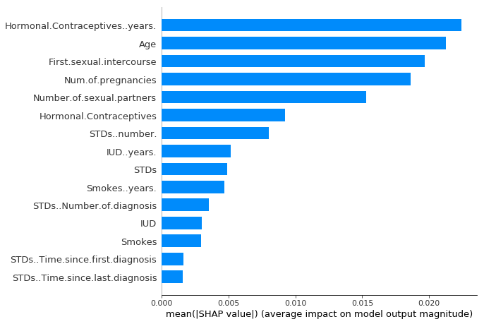
FIGURE 9.25: SHAP feature importance measured as the mean absolute Shapley values. The number of years with hormonal contraceptives was the most important feature, changing the predicted absolute cancer probability on average by 2.4 percentage points (0.024 on x-axis).

SHAP feature importance is an alternative to permutation feature importance. There is a big difference between both importance measures: Permutation feature importance is based on the decrease in model performance. SHAP is based on magnitude of feature attributions.

The feature importance plot is useful, but contains no information beyond the importances. For a more informative plot, we will next look at the summary plot.

SHAP Summary Plot

The summary plot combines feature importance with feature effects. Each point on the summary plot is a Shapley value for a feature and an instance. The position on the y-axis is determined by the feature and on the x-axis by the Shapley value. The color represents the value of the feature from low to high. Overlapping points are jittered in y-axis direction, so we get a sense of the distribution of the Shapley values per feature. The features are ordered according to their importance.

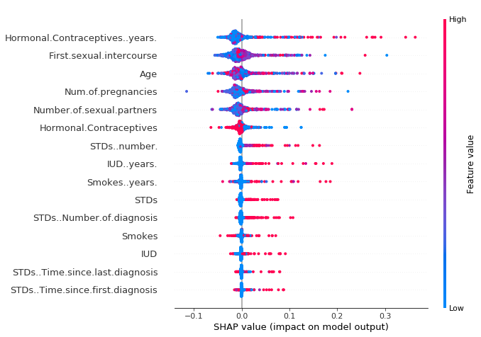
FIGURE 9.26: SHAP summary plot. Low number of years on hormonal contraceptives reduce the predicted cancer risk, a large number of years increases the risk. Your regular reminder: All effects describe the behavior of the model and are not necessarily causal in the real world.

In the summary plot, we see first indications of the relationship between the value of a feature and the impact on the prediction. But to see the exact form of the relationship, we have to look at SHAP dependence plots.

SHAP Dependence Plot

SHAP feature dependence might be the simplest global interpretation plot: 1) Pick a feature. 2) For each data instance, plot a point with the feature value on the x-axis and the corresponding Shapley value on the y-axis. 3) Done.

Mathematically, the plot contains the following points: ${(x_j^{(i)},\phi_j^{(i)})}_{i=1}^n$

The following figure shows the SHAP feature dependence for years on hormonal contraceptives:

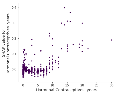
FIGURE 9.27: SHAP dependence plot for years on hormonal contraceptives. Compared to 0 years, a few years lower the predicted probability and a high number of years increases the predicted cancer probability.

SHAP dependence plots are an alternative to partial dependence plots and accumulated local effects. While PDP and ALE plot show average effects, SHAP dependence also shows the variance on the y-axis. Especially in case of interactions, the SHAP dependence plot will be much more dispersed in the y-axis. The dependence plot can be improved by highlighting these feature interactions.

SHAP Interaction Values

The interaction effect is the additional combined feature effect after accounting for the individual feature effects. The Shapley interaction index from game theory is defined as:

when $i\neq{}j$ and:

This formula subtracts the main effect of the features so that we get the pure interaction effect after accounting for the individual effects. We average the values over all possible feature coalitions S, as in the Shapley value computation. When we compute SHAP interaction values for all features, we get one matrix per instance with dimensions M x M, where M is the number of features.

How can we use the interaction index? For example, to automatically color the SHAP feature dependence plot with the strongest interaction:

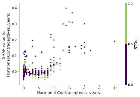
FIGURE 9.28: SHAP feature dependence plot with interaction visualization. Years on hormonal contraceptives interacts with STDs. In cases close to 0 years, the occurence of a STD increases the predicted cancer risk. For more years on contraceptives, the occurence of a STD reduces the predicted risk. Again, this is not a causal model. Effects might be due to confounding (e.g. STDs and lower cancer risk could be correlated with more doctor visits).

Clustering Shapley Values

You can cluster your data with the help of Shapley values. The goal of clustering is to find groups of similar instances. Normally, clustering is based on features. Features are often on different scales. For example, height might be measured in meters, color intensity from 0 to 100 and some sensor output between -1 and 1. The difficulty is to compute distances between instances with such different, non-comparable features.

SHAP clustering works by clustering the Shapley values of each instance. This means that you cluster instances by explanation similarity. All SHAP values have the same unit – the unit of the prediction space. You can use any clustering method. The following example uses hierarchical agglomerative clustering to order the instances.

The plot consists of many force plots, each of which explains the prediction of an instance. We rotate the force plots vertically and place them side by side according to their clustering similarity.

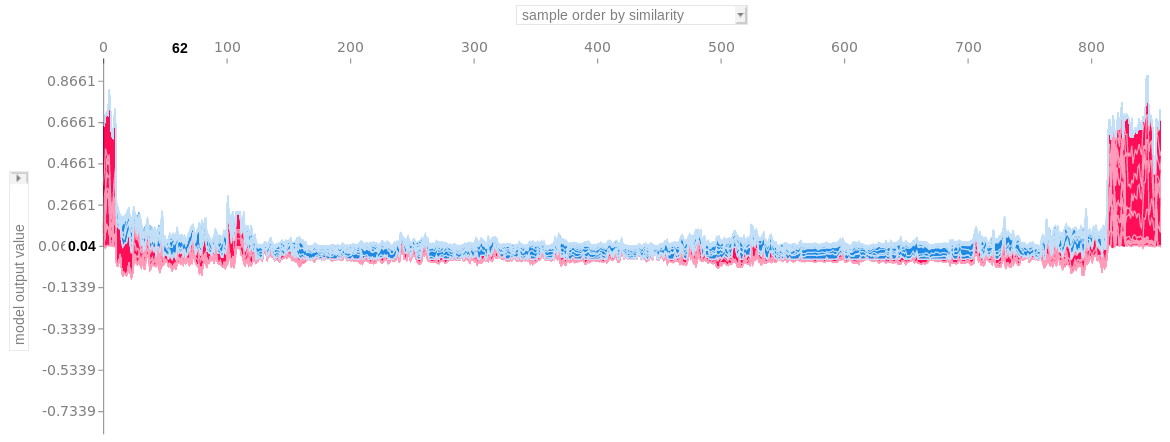
FIGURE 9.29: Stacked SHAP explanations clustered by explanation similarity. Each position on the x-axis is an instance of the data. Red SHAP values increase the prediction, blue values decrease it. One cluster stands out: On the right is a group with a high predicted cancer risk.

Advantages

Since SHAP computes Shapley values, all the advantages of Shapley values apply: SHAP has a solid theoretical foundation in game theory. The prediction is fairly distributed among the feature values. We get contrastive explanations that compare the prediction with the average prediction.

SHAP connects LIME and Shapley values. This is very useful to better understand both methods. It also helps to unify the field of interpretable machine learning.

SHAP has a fast implementation for tree-based models. I believe this was key to the popularity of SHAP, because the biggest barrier for adoption of Shapley values is the slow computation.

The fast computation makes it possible to compute the many Shapley values needed for the global model interpretations. The global interpretation methods include feature importance, feature dependence, interactions, clustering and summary plots. With SHAP, global interpretations are consistent with the local explanations, since the Shapley values are the “atomic unit” of the global interpretations. If you use LIME for local explanations and partial dependence plots plus permutation feature importance for global explanations, you lack a common foundation.

Disadvantages

KernelSHAP is slow. This makes KernelSHAP impractical to use when you want to compute Shapley values for many instances. Also all global SHAP methods such as SHAP feature importance require computing Shapley values for a lot of instances.

KernelSHAP ignores feature dependence. Most other permutation based interpretation methods have this problem. By replacing feature values with values from random instances, it is usually easier to randomly sample from the marginal distribution. However, if features are dependent, e.g. correlated, this leads to putting too much weight on unlikely data points. TreeSHAP solves this problem by explicitly modeling the conditional expected prediction.

TreeSHAP can produce unintuitive feature attributions. While TreeSHAP solves the problem of extrapolating to unlikely data points, it does so by changing the value function and therefore slightly changes the game. TreeSHAP changes the value function by relying on the conditional expected prediction. With the change in the value function, features that have no influence on the prediction can get a TreeSHAP value different from zero.

The disadvantages of Shapley values also apply to SHAP: Shapley values can be misinterpreted and access to data is needed to compute them for new data (except for TreeSHAP).

It is possible to create intentionally misleading interpretations with SHAP, which can hide biases 73. If you are the data scientist creating the explanations, this is not an actual problem (it would even be an advantage if you are the evil data scientist who wants to create misleading explanations). For the receivers of a SHAP explanation, it is a disadvantage: they cannot be sure about the truthfulness of the explanation.

Software

The authors implemented SHAP in the shap Python package. This implementation works for tree-based models in the scikit-learn machine learning library for Python. The shap package was also used for the examples in this chapter. SHAP is integrated into the tree boosting frameworks xgboost and LightGBM. In R, there are the shapper and fastshap packages. SHAP is also included in the R xgboost package.