ML - Gradient Boosting Algorithm
Introduction
Gradient boosting is one of the variants of ensemble methods where you create multiple weak models and combine them to get better performance as a whole.
Gradient boosting is one of the most powerful techniques for building predictive models.
The Origin of Boosting
The idea of boosting came out of the idea of whether a weak learner can be modified to become better.
Michael Kearns articulated the goal as the “Hypothesis Boosting Problem” stating the goal from a practical standpoint as:
… an efficient algorithm for converting relatively poor hypotheses into very good hypotheses
— Thoughts on Hypothesis Boosting [PDF], 1988
A weak hypothesis or weak learner is defined as one whose performance is at least slightly better than random chance.
These ideas built upon Leslie Valiant’s work on distribution free or Probably Approximately Correct (PAC) learning, a framework for investigating the complexity of machine learning problems.
Hypothesis boosting was the idea of filtering observations, leaving those observations that the weak learner can handle and focusing on developing new weak learns to handle the remaining difficult observations.
The idea is to use the weak learning method several times to get a succession of hypotheses, each one refocused on the examples that the previous ones found difficult and misclassified. … Note, however, it is not obvious at all how this can be done
— Probably Approximately Correct: Nature’s Algorithms for Learning and Prospering in a Complex World, page 152, 2013
AdaBoost the First Boosting Algorithm
The first realization of boosting that saw great success in application was Adaptive Boosting or AdaBoost for short.
Boosting refers to this general problem of producing a very accurate prediction rule by combining rough and moderately inaccurate rules-of-thumb.
— A decision-theoretic generalization of on-line learning and an application to boosting [PDF], 1995
The weak learners in AdaBoost are decision trees with a single split, called decision stumps for their shortness.
AdaBoost works by weighting the observations, putting more weight on difficult to classify instances and less on those already handled well. New weak learners are added sequentially that focus their training on the more difficult patterns.
This means that samples that are difficult to classify receive increasing larger weights until the algorithm identifies a model that correctly classifies these samples
— Applied Predictive Modeling, 2013
Predictions are made by majority vote of the weak learners’ predictions, weighted by their individual accuracy. The most successful form of the AdaBoost algorithm was for binary classification problems and was called AdaBoost.M1.
You can learn more about the AdaBoost algorithm in the post:
Generalization of AdaBoost as Gradient Boosting
AdaBoost and related algorithms were recast in a statistical framework first by Breiman calling them ARCing algorithms.
Arcing is an acronym for Adaptive Reweighting and Combining. Each step in an arcing algorithm consists of a weighted minimization followed by a recomputation of [the classifiers] and [weighted input].
— Prediction Games and Arching Algorithms [PDF], 1997
This framework was further developed by Friedman and called Gradient Boosting Machines. Later called just gradient boosting or gradient tree boosting.
The statistical framework cast boosting as a numerical optimization problem where the objective is to minimize the loss of the model by adding weak learners using a gradient descent like procedure.
This class of algorithms were described as a stage-wise additive model. This is because one new weak learner is added at a time and existing weak learners in the model are frozen and left unchanged.
Note that this stagewise strategy is different from stepwise approaches that readjust previously entered terms when new ones are added.
— Greedy Function Approximation: A Gradient Boosting Machine [PDF], 1999
The generalization allowed arbitrary differentiable loss functions to be used, expanding the technique beyond binary classification problems to support regression, multi-class classification and more.
How Gradient Boosting Works
Gradient boosting involves three elements:
- A loss function to be optimized.
- A weak learner to make predictions.
- An additive model to add weak learners to minimize the loss function.
1. Loss Function
The loss function used depends on the type of problem being solved.
It must be differentiable, but many standard loss functions are supported and you can define your own.
For example, regression may use a squared error and classification may use logarithmic loss.
A benefit of the gradient boosting framework is that a new boosting algorithm does not have to be derived for each loss function that may want to be used, instead, it is a generic enough framework that any differentiable loss function can be used.
2. Weak Learner
Decision trees are used as the weak learner in gradient boosting.
Specifically regression trees are used that output real values for splits and whose output can be added together, allowing subsequent models outputs to be added and “correct” the residuals in the predictions.
Trees are constructed in a greedy manner, choosing the best split points based on purity scores like Gini or to minimize the loss.
Initially, such as in the case of AdaBoost, very short decision trees were used that only had a single split, called a decision stump. Larger trees can be used generally with 4-to-8 levels.
It is common to constrain the weak learners in specific ways, such as a maximum number of layers, nodes, splits or leaf nodes.
This is to ensure that the learners remain weak, but can still be constructed in a greedy manner.
3. Additive Model
Trees are added one at a time, and existing trees in the model are not changed.
A gradient descent procedure is used to minimize the loss when adding trees.
Traditionally, gradient descent is used to minimize a set of parameters, such as the coefficients in a regression equation or weights in a neural network. After calculating error or loss, the weights are updated to minimize that error.
Instead of parameters, we have weak learner sub-models or more specifically decision trees. After calculating the loss, to perform the gradient descent procedure, we must add a tree to the model that reduces the loss (i.e. follow the gradient). We do this by parameterizing the tree, then modify the parameters of the tree and move in the right direction by (reducing the residual loss.
Generally this approach is called functional gradient descent or gradient descent with functions.
One way to produce a weighted combination of classifiers which optimizes [the cost] is by gradient descent in function space
— Boosting Algorithms as Gradient Descent in Function Space [PDF], 1999
The output for the new tree is then added to the output of the existing sequence of trees in an effort to correct or improve the final output of the model.
A fixed number of trees are added or training stops once loss reaches an acceptable level or no longer improves on an external validation dataset.
Improvements to Basic Gradient Boosting
Gradient boosting is a greedy algorithm and can overfit a training dataset quickly.
It can benefit from regularization methods that penalize various parts of the algorithm and generally improve the performance of the algorithm by reducing overfitting.
In this this section we will look at 4 enhancements to basic gradient boosting:
- Tree Constraints
- Shrinkage
- Random sampling
- Penalized Learning
1. Tree Constraints
It is important that the weak learners have skill but remain weak.
There are a number of ways that the trees can be constrained.
A good general heuristic is that the more constrained tree creation is, the more trees you will need in the model, and the reverse, where less constrained individual trees, the fewer trees that will be required.
Below are some constraints that can be imposed on the construction of decision trees:
- Number of trees, generally adding more trees to the model can be very slow to overfit. The advice is to keep adding trees until no further improvement is observed.
- Tree depth, deeper trees are more complex trees and shorter trees are preferred. Generally, better results are seen with 4-8 levels.
- Number of nodes or number of leaves, like depth, this can constrain the size of the tree, but is not constrained to a symmetrical structure if other constraints are used.
- Number of observations per split imposes a minimum constraint on the amount of training data at a training node before a split can be considered
- Minimim improvement to loss is a constraint on the improvement of any split added to a tree.
2. Weighted Updates
The predictions of each tree are added together sequentially.
The contribution of each tree to this sum can be weighted to slow down the learning by the algorithm. This weighting is called a shrinkage or a learning rate.
Each update is simply scaled by the value of the “learning rate parameter v”
— Greedy Function Approximation: A Gradient Boosting Machine [PDF], 1999
The effect is that learning is slowed down, in turn require more trees to be added to the model, in turn taking longer to train, providing a configuration trade-off between the number of trees and learning rate.
Decreasing the value of v [the learning rate] increases the best value for M [the number of trees].
— Greedy Function Approximation: A Gradient Boosting Machine [PDF], 1999
It is common to have small values in the range of 0.1 to 0.3, as well as values less than 0.1.
Similar to a learning rate in stochastic optimization, shrinkage reduces the influence of each individual tree and leaves space for future trees to improve the model.
— Stochastic Gradient Boosting [PDF], 1999
3. Stochastic Gradient Boosting
A big insight into bagging ensembles and random forest was allowing trees to be greedily created from subsamples of the training dataset.
This same benefit can be used to reduce the correlation between the trees in the sequence in gradient boosting models.
This variation of boosting is called stochastic gradient boosting.
at each iteration a subsample of the training data is drawn at random (without replacement) from the full training dataset. The randomly selected subsample is then used, instead of the full sample, to fit the base learner.
— Stochastic Gradient Boosting [PDF], 1999
A few variants of stochastic boosting that can be used:
- Subsample rows before creating each tree.
- Subsample columns before creating each tree
- Subsample columns before considering each split.
Generally, aggressive sub-sampling such as selecting only 50% of the data has shown to be beneficial.
According to user feedback, using column sub-sampling prevents over-fitting even more so than the traditional row sub-sampling
— XGBoost: A Scalable Tree Boosting System, 2016
4. Penalized Gradient Boosting
Additional constraints can be imposed on the parameterized trees in addition to their structure.
Classical decision trees like CART are not used as weak learners, instead a modified form called a regression tree is used that has numeric values in the leaf nodes (also called terminal nodes). The values in the leaves of the trees can be called weights in some literature.
As such, the leaf weight values of the trees can be regularized using popular regularization functions, such as:
- L1 regularization of weights.
- L2 regularization of weights.
The additional regularization term helps to smooth the final learnt weights to avoid over-fitting. Intuitively, the regularized objective will tend to select a model employing simple and predictive functions.
— XGBoost: A Scalable Tree Boosting System, 2016
Gradient Boosting Resources
Gradient boosting is a fascinating algorithm and I am sure you want to go deeper.
This section lists various resources that you can use to learn more about the gradient boosting algorithm.
Gradient Boosting Videos
- Gradient Boosting Machine Learning, Trevor Hastie, 2014
- Gradient Boosting, Alexander Ihler, 2012
- GBM, John Mount, 2015
- Learning: Boosting, MIT 6.034 Artificial Intelligence, 2010
- xgboost: An R package for Fast and Accurate Gradient Boosting, 2016
- XGBoost: A Scalable Tree Boosting System, Tianqi Chen, 2016
Gradient Boosting in Textbooks
- Section 8.2.3 Boosting, page 321, An Introduction to Statistical Learning: with Applications in R.
- Section 8.6 Boosting, page 203, Applied Predictive Modeling.
- Section 14.5 Stochastic Gradient Boosting, page 390, Applied Predictive Modeling.
- Section 16.4 Boosting, page 556, Machine Learning: A Probabilistic Perspective
- Chapter 10 Boosting and Additive Trees, page 337, The Elements of Statistical Learning: Data Mining, Inference, and Prediction
Gradient Boosting Papers
- Thoughts on Hypothesis Boosting [PDF], Michael Kearns, 1988
- A decision-theoretic generalization of on-line learning and an application to boosting [PDF], 1995
- Arcing the edge [PDF], 1998
- Stochastic Gradient Boosting [PDF], 1999
- Boosting Algorithms as Gradient Descent in Function Space [PDF], 1999
Gradient Boosting Slides
Gradient Boosting Web Pages
Summary
In this post you discovered the gradient boosting algorithm for predictive modeling in machine learning.
Specifically, you learned:
- The history of boosting in learning theory and AdaBoost.
- How the gradient boosting algorithm works with a loss function, weak learners and an additive model.
- How to improve the performance of gradient boosting with regularization.
Tomonori Masui’ post
Cliped from Towards Data Science All You Need to Know about Gradient Boosting Algorithm − Part 1. Regression
Section 1. Algorithm with an Example
Gradient boosting is one of the most popular machine learning algorithms for tabular datasets. It is powerful enough to find any nonlinear relationship between your model target and features and has great usability that can deal with missing values, outliers, and high cardinality categorical values on your features without any special treatment. While you can build barebone gradient boosting trees using some popular libraries such as XGBoost or LightGBM without knowing any details of the algorithm, you still want to know how it works when you start tuning hyper-parameters, customizing the loss functions, etc., to get better quality on your model.
This article aims to provide you with all the details about the algorithm, specifically its regression algorithm, including its math and Python code from scratch. If you are more interested in the classification algorithm, please look at Part 2.
Gradient boosting is one of the variants of ensemble methods where you create multiple weak models and combine them to get better performance as a whole.
In this section, we are building gradient boosting regression trees step by step using the below sample which has a nonlinear relationship between $x$ and $y$ to intuitively understand how it works (all the pictures below are created by the author).

The first step is making a very naive prediction on the target $y$. We make the initial prediction $F_0$ as an overall average of $y$:
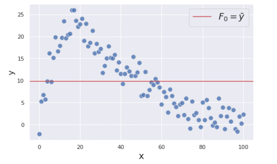
You might feel using the mean for the prediction is silly, but don’t worry. We will improve our prediction as we add more weak models to it.
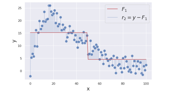
To improve our prediction, we will focus on the residuals (i.e. prediction errors) from the first step because that is what we want to minimize to get a better prediction. The residuals $r₁$ are shown as the vertical blue lines in the figure below.

To minimize these residuals, we are building a regression tree model with $x$ as its feature and the residuals $r_1 = y − \text{mean}(y)$ as its target. The reasoning behind that is if we can find some patterns between $x$ and $r_1$ by building the additional weak model, we can reduce the residuals by utilizing it.
To simplify the demonstration, we are building very simple trees each of that only has one split and two terminal nodes which is called “stump”. Please note that gradient boosting trees usually have a little deeper trees such as ones with 8 to 32 terminal nodes.
Here we are creating the first tree predicting the residuals with two different values $\gamma _1 = {6.0, − 5.9}$(we are using $\gamma$ (gamma) to denotes the prediction).

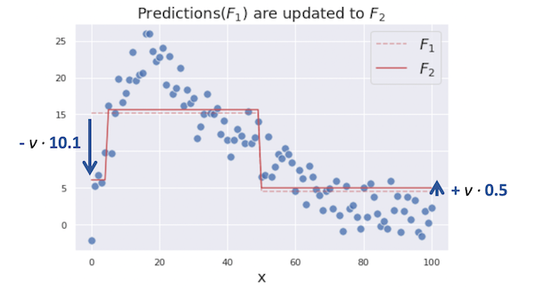
This prediction $\gamma _1$ is added to our initial prediction $F_0$ to reduce the residuals. In fact, gradient boosting algorithm does not simply add $\gamma$ to $F$ as it makes the model overfit to the training data. Instead, $\gamma$ is scaled down by learning rate $\nu$ which ranges between 0 and 1, and then added to $F$.
\[F_1 = F_0 + \nu \cdot \gamma _1\]In this example, we use a relatively big learning rate $\nu = 0.9$ to make the optimization process easier to understand, but it is usually supposed to be a much smaller value such as 0.1.
After the update, our combined prediction $F_1$ becomes:
\[F_1 = \begin{cases} F_0 + \nu \cdot 6.0 &\text{if } x \leq 49.5 \\ F_0 - \nu \cdot 5.9 &\text{otherwise} \end{cases}\]Now, the updated residuals $r_2$ looks like this:
In the next step, we are creating a regression tree again using the same $x$ as the feature and the updated residuals $r_2$ as its target. Here is the created tree:

Then, we are updating our previous combined prediction $F_1$ with the new tree prediction $\gamma _2$.
We iterate these steps until the model prediction stops improving. The figures below show the optimization process from 0 to 6 iterations.

You can see the combined prediction $F_m$ is getting more closer to our target $y$ as we add more trees into the combined model. This is how gradient boosting works to predict complex targets by combining multiple weak models.
Section 2. Math
In this section, we are diving into the math details of the algorithm. Here is the whole algorithm in math formulas.
 Source: adapted from Wikipedia and Friedman’s paper
Let’s demystify this line by line.
Step 1
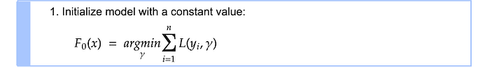
The first step is creating an initial constant value prediction $F_0$. $L$ is the loss function and it is squared loss in our regression case.

$argmin$ means we are searching for the value $\gamma$ that minimizes $\sum L(y_i, \gamma)$. Let’s compute the value $\gamma$ by using our actual loss function. To find $\gamma$ that minimizes $ΣL$, we are taking a derivative of $\sum L$ with respect to $\gamma$.
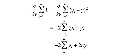
And we are finding $\gamma$ that makes $\frac {\partial \sum L} {\gamma}$ equal to 0.

It turned out that the value $\gamma$ that minimizes $ΣL$ is the mean of $y$. This is why we used $y$ mean for our initial prediction $F₀$ in the last section.

Step2

The whole step2 processes from 2–1 to 2–4 are iterated $M$ times. $M$ denotes the number of trees we are creating and the small $m$ represents the index of each tree.
Step 2–1

We are calculating residuals $r_i 𝑚$ by taking a derivative of the loss function with respect to the previous prediction $F_{m-1}$ and multiplying it by −1. As you can see in the subscript index, $r_i m$ is computed for each single sample $i$. Some of you might be wondering why we are calling this $rᵢ𝑚$ residuals. This value is actually negative gradient that gives us guidance on the directions ($+/−$) and the magnitude in which the loss function can be minimized. You will see why we are calling it residuals shortly. By the way, this technique where you use a gradient to minimize the loss on your model is very similar to gradient descent technique which is typically used to optimize neural networks. (In fact, they are slightly different from each other. If you are interested, please look at this article detailing that topic.)
Let’s compute the residuals here. $F{m-1}$ in the equation means the prediction from the previous step. In this first iteration, it is $F_0$. We are solving the equation for residuals $r_i 𝑚$.

We can take 2 out of it as it is just a constant. That leaves us $r_{im} = y_i − F_{m-1}$. You might now see why we call it residuals. This also gives us interesting insight that the negative gradient that provides us the direction and the magnitude to which the loss is minimized is actually just residuals.
Step 2–2

$j$ represents a terminal node (i.e. leave) in the tree, $m$ denotes the tree index, and capital $J$ means the total number of leaves.
Step 2–3

We are searching for $\gamma {jm}$ that minimizes the loss function on each terminal node $j$. $\sum x_i R{jm} L$ means we are aggregating the loss on all the sample $x_i$s that belong to the terminal node $R_{im}$. Let’s plugin the loss function into the equation.
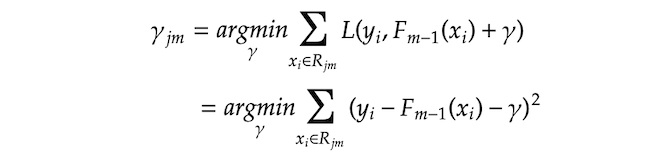
Then, we are finding $\gamma _{jm}$ that makes the derivative of $\sum (*)$ equals zero.

Please note that $n_j$ means the number of samples in the terminal node $j$. This means the optimal $\gamma {jm}$ that minimizes the loss function is the average of the residuals $r{im}$ in the terminal node $R_j m$. In other words, $\gamma _{jm}$ is the regular prediction values of regression trees that are the average of the target values (in our case, residuals) in each terminal node.
Step 2–4

In the final step, we are updating the prediction of the combined model $F_m$. $\gamma {jm} 1(x ∈ R{jm})$ means that we pick the value $\gamma {im}$ if a given $x$ falls in a terminal node $R{jm}$. As all the terminal nodes are exclusive, any given single $x$ falls into only a single terminal node and corresponding $\gammaⱼ𝑚$ is added to the previous prediction $F_{m-1}_$ and it makes updated prediction $F_m$.
As mentioned in the previous section, $\nu$ is learning rate ranging between 0 and 1 which controls the degree of contribution of the additional tree prediction $\gamma$ to the combined prediction $F_m$. A smaller learning rate reduces the effect of the additional tree prediction, but it basically also reduces the chance of the model overfitting to the training data.
Now we have gone through the whole steps. To get the best model performance, we want to iterate step 2 $M$ times, which means adding $M$ trees to the combined model. In reality, you might often want to add more than 100 trees to get the best model performance.
Some of you might feel that all those maths are unnecessarily complex as the previous section showed the basic idea in a much simpler way without all those complications. The reason behind it is that gradient boosting is designed to be able to deal with any loss functions as long as it is differentiable and the maths we reviewed is a generalized form of gradient boosting algorithm with that flexibility. That makes the formula a little complex, but it is the beauty of the algorithm as it has huge flexibility and convenience to work on a variety of types of problems. For example, if your problem requires absolute loss instead of squared loss, you can just replace the loss function and the whole algorithm works as it is as defined above. In fact, popular gradient boosting implementations such as XGBoost or LightGBM have a wide variety of loss functions, so you can choose whatever loss functions that suit your problem (see the various loss functions available in XGBoost or LightGBM).
Section 3. Code
In this section, we are translating the maths we just reviewed into a viable python code to help us understand the algorithm further. The code is mostly derived from Matt Bowers’ implementation, so all credit goes to his work. We are using DecisionTreeRegressor from scikit-learn to build trees which helps us just focus on the gradient boosting algorithm itself instead of the tree algorithm. We are imitating scikit-learn style implementation where you train the model with fit method and make predictions with predict method.
class CustomGradientBoostingRegressor:

    def __init__(self, learning_rate, n_estimators, max_depth=1):
        self.learning_rate = learning_rate
        self.n_estimators = n_estimators
        self.max_depth = max_depth
        self.trees = []

    def fit(self, X, y):

        self.F0 = y.mean()
        Fm = self.F0

        for _ in range(self.n_estimators):
            r = y - Fm
            tree = DecisionTreeRegressor(max_depth=self.max_depth, random_state=0)
            tree.fit(X, r)
            gamma = tree.predict(X)
            Fm += self.learning_rate * gamma
            self.trees.append(tree)

    def predict(self, X):

        Fm = self.F0

        for i in range(self.n_estimators):
            Fm += self.learning_rate * self.trees[i].predict(X)

        return Fm
Please note that all the trained trees are stored in self.trees list object and it is retrieved when we make predictions with predict method.
Next, we are checking if our CustomGradientBoostingRegressor performs as the same as GradientBoostingRegressor from scikit-learn by looking at their RMSE on our data.
from sklearn.ensemble import GradientBoostingRegressor
from sklearn.metrics import mean_squared_error

custom_gbm = CustomGradientBoostingRegressor(
    n_estimators=20,
    learning_rate=0.1,
    max_depth=1
)
custom_gbm.fit(x, y)
custom_gbm_rmse = mean_squared_error(y, custom_gbm.predict(x), squared=False)
print(f"Custom GBM RMSE:{custom_gbm_rmse:.15f}")

sklearn_gbm = GradientBoostingRegressor(
    n_estimators=20,
    learning_rate=0.1,
    max_depth=1
)
sklearn_gbm.fit(x, y)
sklearn_gbm_rmse = mean_squared_error(y, sklearn_gbm.predict(x), squared=False)
print(f"Scikit-learn GBM RMSE:{sklearn_gbm_rmse:.15f}")
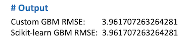
As you can see in the output above, both models have exactly the same RMSE.
The algorithm we have reviewed in this post is just one of the options of gradient boosting algorithm that is specific to regression problems with squared loss. If you are also interested in the classification algorithm, please look at Part 2.
There are also some other great resources if you want further details of the algorithm:
- StatQuest, Gradient Boost Part1 and Part 2
This is a YouTube video explaining GB regression algorithm with great visuals in a beginner-friendly way. - Terence Parr and Jeremy Howard, How to explain gradient boostingThis article also focuses on GB regression. It explains how the algorithms differ between squared loss and absolute loss.
- Jerome Friedman, Greedy Function Approximation: A Gradient Boosting MachineThis is the original paper from Friedman. While it is a little hard to understand, it surely shows the flexibility of the algorithm where he shows a generalized algorithm that can deal with any types of problem having a differentiable loss function.
You can also look at the full Python code in the Google Colab link or the Github link below.
- Jerome Friedman, Greedy Function Approximation: A Gradient Boosting Machine
- Terence Parr and Jeremy Howard, How to explain gradient boosting
- Matt Bowers, How to Build a Gradient Boosting Machine from Scratch
- Wikipedia, Gradient boosting